6. Reading and plotting with xarray
6.1. Synopsis
- Use xarray to read and plot spherical data in only a few lines
6.2. xarray
We now turn to the package xarray whose documentation you can find at http://xarray.pydata.org/en/stable/index.html.
Install with
conda install -c conda-forge xarray
although you should check their documentation for other dependencies such as cartopy (we’ve used the critical ones in earlier notebooks so if you’ve been following along you should be alright).
Here’s the usual import cell:
[1]:
import xarray
import cartopy.crs
import matplotlib.pyplot as plt
In terms of what we’ve already covered, xarray plays the role of the netCDF4 and matplotlib.pyplot packages combined. It allows us to open a dataset and plot it with minimal intermediate steps.
First, we’ll open the same dataset that we earlier accessed using netCDF4.Dataset() but this time with xarray.open_dataset():
[2]:
ds = xarray.open_dataset('http://esgf-data2.diasjp.net/thredds/dodsC/esg_dataroot/CMIP6/CMIP/MIROC/MIROC6/1pctCO2/r1i1p1f1/Omon/tos/gn/v20181212/tos_Omon_MIROC6_1pctCO2_r1i1p1f1_gn_330001-334912.nc')
C:\Users\ajadc\Miniconda3\envs\py3\lib\site-packages\xarray\coding\times.py:122: SerializationWarning: Unable to decode time axis into full numpy.datetime64 objects, continuing using dummy cftime.datetime objects instead, reason: dates out of range
  result = decode_cf_datetime(example_value, units, calendar)
C:\Users\ajadc\Miniconda3\envs\py3\lib\site-packages\xarray\coding\variables.py:69: SerializationWarning: Unable to decode time axis into full numpy.datetime64 objects, continuing using dummy cftime.datetime objects instead, reason: dates out of range
  return self.func(self.array)
If you see pink-background warnings, don’t worry - that’s a result of the choice of dataset. The dataset was opened and we can query it by looking at the variable, ds, we created:
[3]:
print(ds)
<xarray.Dataset>
Dimensions:             (bnds: 2, time: 600, vertices: 4, x: 360, y: 256)
Coordinates:
  * time                (time) object 3300-01-16 12:00:00 ... 3349-12-16 12:00:00
  * y                   (y) float64 -88.0 -85.75 -85.25 ... 148.6 150.5 152.4
  * x                   (x) float64 0.5 1.5 2.5 3.5 ... 356.5 357.5 358.5 359.5
    latitude            (y, x) float32 ...
    longitude           (y, x) float32 ...
Dimensions without coordinates: bnds, vertices
Data variables:
    time_bnds           (time, bnds) object ...
    y_bnds              (y, bnds) float64 ...
    x_bnds              (x, bnds) float64 ...
    vertices_latitude   (y, x, vertices) float32 ...
    vertices_longitude  (y, x, vertices) float32 ...
    tos                 (time, y, x) float32 ...
Attributes:
    _NCProperties:                   version=1|netcdflibversion=4.6.1|hdf5lib...
    Conventions:                     CF-1.7 CMIP-6.2
    activity_id:                     CMIP
    branch_method:                   standard
    branch_time_in_child:            0.0
    branch_time_in_parent:           0.0
    creation_date:                   2018-11-30T13:31:08Z
    data_specs_version:              01.00.28
    experiment:                      1 percent per year increase in CO2
    experiment_id:                   1pctCO2
    external_variables:              areacello
    forcing_index:                   1
    frequency:                       mon
    further_info_url:                https://furtherinfo.es-doc.org/CMIP6.MIR...
    grid:                            native ocean tripolar grid with 360x256 ...
    grid_label:                      gn
    history:                         2018-11-30T13:31:08Z ; CMOR rewrote data...
    initialization_index:            1
    institution:                     JAMSTEC (Japan Agency for Marine-Earth S...
    institution_id:                  MIROC
    mip_era:                         CMIP6
    nominal_resolution:              100 km
    parent_activity_id:              CMIP
    parent_experiment_id:            piControl
    parent_mip_era:                  CMIP6
    parent_source_id:                MIROC6
    parent_time_units:               days since 3200-1-1
    parent_variant_label:            r1i1p1f1
    physics_index:                   1
    product:                         model-output
    realization_index:               1
    realm:                           ocean
    source:                          MIROC6 (2017): \naerosol: SPRINTARS6.0\n...
    source_id:                       MIROC6
    source_type:                     AOGCM AER
    sub_experiment:                  none
    sub_experiment_id:               none
    table_id:                        Omon
    table_info:                      Creation Date:(06 November 2018) MD5:072...
    title:                           MIROC6 output prepared for CMIP6
    variable_id:                     tos
    variant_label:                   r1i1p1f1
    license:                         CMIP6 model data produced by MIROC is li...
    cmor_version:                    3.3.2
    tracking_id:                     hdl:21.14100/636faabd-555e-414a-bbba-e25...
    DODS_EXTRA.Unlimited_Dimension:  time
This is the same information we saw when we printed the netCDF4.Dataset object except that this time it is much easier to read and at the same time is more concise!
The coordinates section is of particular interest. Dimension variables (defined in Basics of accessing data) are indicated with an asterisk (“*”) but there are some 2D variables in the coordinate section too.
We still have to use cartopy as before to handle spherical coordinates but to make a plot we need only two statements: 1. Specify the projection (otherwise how would python know how you want to look at the data?) 2. Specify the data to plot (ds.tos[0])
[4]:
ax = plt.axes(projection=cartopy.crs.Robinson());
ds.tos[0].plot(transform=cartopy.crs.PlateCarree(), x='longitude', y='latitude');
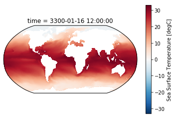
Notice how the time of the dataset was kindly added to the plot? This is an example of the convenience of a high-level package relative to the lower-level operations we’ve been using via netCDF4 and matplotlib.pyplot. xarray is designed for intuitive analysis of N-dimensional data.
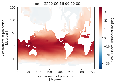
To be complete, if you wish to skip the projection and plot using the projection coordinates, viewing the data with fully labeled axes and colorbar is as easy as this one line:
[5]:
ds.tos[5].plot();
6.3. Summary
- xarray is a high-level layer that sits on top of netCDF4 (or other APIs) and matplotlib.
- Used
.plot()with cartopy to plot in just two lines.